Deep Learning

Deep learning. It seems to be all the rage these days. But what is it? Sure, we all know there is some model, some data, some computations, some magic, and... you get Chat-GPT. Great, but how do all these seemingly unrelated concepts work together? Does this model walk down a runway? What do we do with the data? And most importantly - how easy it is for you to do the same magic.

Deep Dive into Deep Learning

Deep Learning is by no means a new concept. Since the 60s researches have been exploring the concept of utilising machines to automatically identify visual characters [1] [2]. It built upon existing Machine Learning techniques, by introducing non-linearity for more complex problems. As we saw in the introductory article on Machine Learning, the simplest model to exist is linear regression:

Extended to multiple dimensions (where y and x are not just a single value, but house multiple ones), the equation becomes:

Where M is matrix. This is a lot of complex Linear Algebra to calculate the following:

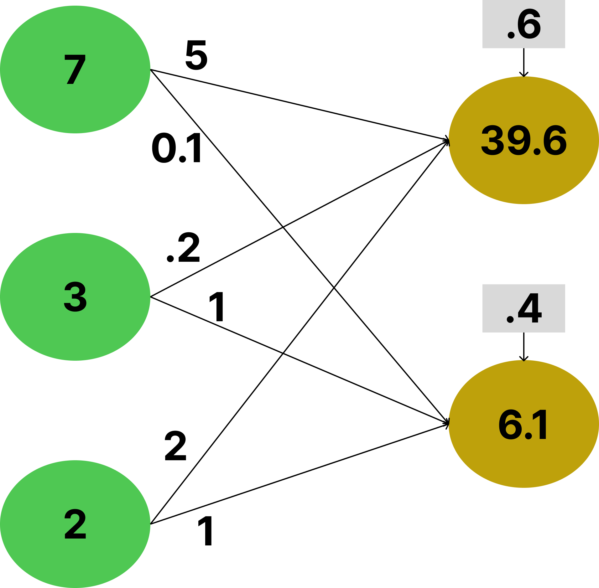
In green we see the input vector (x) and its three values. On the lines we see the values of the matrix M. In gray boxes above the red circles we see the values of the bias vector (b). In red we see the output (y). For each line we multiply the value from where it originates with the value on the line. We add up all the values in the destination circle, where when we add the bias term (above it), we get the result of the output.

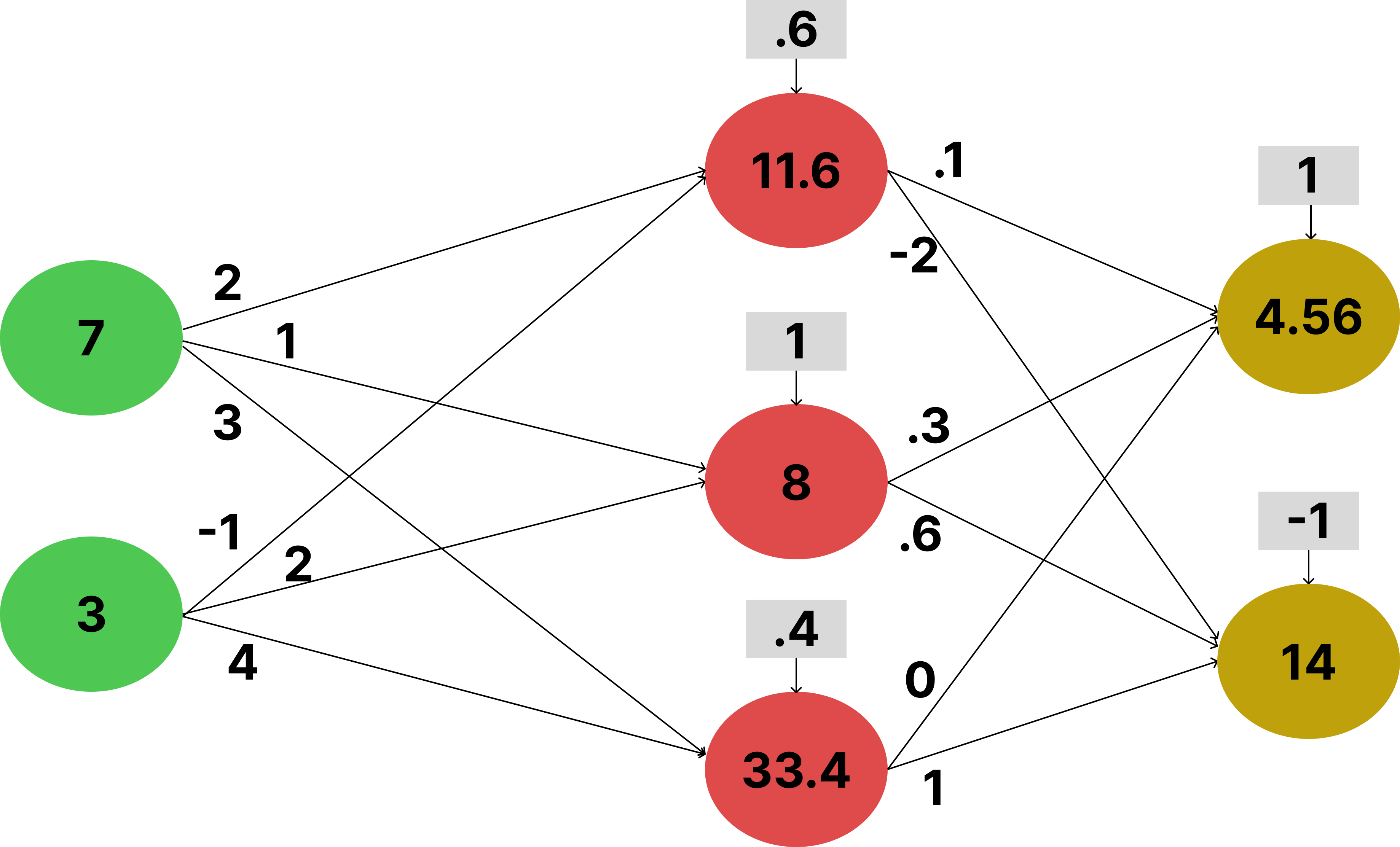
This is the foundation of Deep Learning - the neural network. The circles are the "neurons" and the connecting lines specify how one affects the other. The simplest such network (Multilayer perceptron) takes the form of multiple such multiplication calculations:

Or presented visually:

Where the non-linear-activation() is some function that breaks away from the linearity of Mx + b. The simplest example is the Rectified Linear Unit (ReLU), which given some input vector x, per element makes the values positive (if not already).

You can have any number of layers going "deeper", forming the hidden layers of a network (those between the input and the output calculation), typically expressed as h(x):

And this is essentially what Neural Networks are. A series of independent calculations, where the input to a layer is the output of the previous one. They are modular and thus easy to swap out/change, while trying different models. And, given enough linear layers and data, one can approximate any function with a Multi-Layer perceptron.

You can play around with a 2-layer Multi-perceptron in the interactive example below. For simplicity's sake the bias vectors have been removed. Also certain connections are omitted as it would be too cluttered visually. Click on any of the numbers on the lines to change the given activation's value and see how this affects the final output:

Training the Model

If one were to just create some arbitrary neural network, it would be a bit surprising if by sheer chance the initial parameters selected at random were able to perform the task at hand. Usually (for those of us not so lucky), a model needs to be first trained on data relevant to the task, before it could perform with satisfactory results. The typical training cycle (called Stochastic Gradient Descent, SGD for short [3]) for a neural network proceeds as follows:

1. Raw data is sampled and fed to the input layer
2. Intermediate layers perform computations based on the output from the previous layer x and their weights W, and provide their output as input to the subsequent one y
3. The last layers provides a final output output
4. A relevant loss function 𝓛 is used which computes how "inaccurate" the result was given some target - loss = 𝓛(target,output)
5. This loss is fed back into the last layer
6. Each layer computes an update (gradient) for each of their weights $\frac{\delta \mathrm{y}}{\delta \mathrm{W}}$ based on the gradient input (δy) from the next layer (as this time the flow is in reverse) and provides the previous layer with the gradient of its forward input $\frac{\delta \mathrm{y}}{\delta \mathrm{x}}$. For the last layer, the input it gets during this step is the result of the loss function.
7. Weights are updated with W = W - $\lambda \frac{\delta \mathrm{y}}{\delta \mathrm{W}}$ where λ is a small constant representing the learning rate.

The last two steps of the process constitute the backpropagation algorithm [4] - an efficient application of the chain rule. This algorithm finds the change needed for each parameter in order for, given an input, the network can approximate better the target output. This small adjustment of parameters is performed in the last step, W = W - $\frac{\delta \mathrm{y}}{\delta \mathrm{W}}$. This $\lambda \frac{\delta \mathrm{y}}{\delta \mathrm{W}}$ is exactly the change needed by each parameter in order for the network to improve its predictions. The backpropagation algorithm merely facilitates computation of this change across the different modules/layers, by needing from them only to compute their local change $\frac{\delta \mathrm{y}}{\delta \mathrm{W}}$ and the error with respect to its input x, which is fed to the previous layer as its y: $\frac{\delta \mathrm{y}}{\delta \mathrm{x}}$. Thus when building these complex neural network that reach billions of parameters in size [5], you don't need to write each time an algorithm through which the error can be corrected for your specific architecture. A lot of this has been abstracted away in modern packages like Torch or TensorFlow, where you can build a neural network with any combination of layers, feed it data, compute some loss, and it will automatically compute the updates for each weight.

To conclude, the training cycle can be seen as a loop of 5 steps - getting data, forward pass, loss computation, backward pass, weight updates.

Unsupervised and Reinforcement Learning

While the above example focused on Supervised Learning, you can just as easily apply Deep Learning for both Unsupervised and Reinforcement Learning. All you need to change is what loss is used. GANs or Generative Adversarial Networks are the most common example of unsupervised learning. But there are also Autoencoders, Diffusion Networks, and Anomaly Detection.

Representation Learning

Deep Learning can also be thought of as "representation" learning. The goal is given raw input to automatically extract meaningful features. Before Deep Neural Networks, you would typically need to identify manually features and translate them into some scalar. So for example if you were trying to determine if something is a cat or dog based on an image, you would need to preprocess it and extract some useful information from it (distance between eyes and nose, shape of ears...). With Deep Learning you feed the raw data to the network and it learns a representation (the features) from it. The hidden layers learn some abstract representation of your data, simplifying it into some n-dimensional feature that is learnt from the data, and is then used to perform the final classification (example dog or cat) on the very last output layer.